
Aust J Crop Sci. 19(01):69-75 (2025) | ISSN:1835-2707
https://doi.org/10.21475/ajcs.25.19.01.p194
The impact of climactic and spectral variables on soybean productivity: An approach to spatial panel data
Edilza Martins Silva*1, Alex Paludo1, Willyan Ronaldo Becker1, Priscila Pigatto Gasparin2, Luciana Pagliosa Carvalho Guedes1, Jerry Adriani Johann1
1Western Paraná State University, (UNIOESTE), Cascavel, Paraná, Brazil
2Federal University of Technology, Paraná (UTFPR), Medianeira, Paraná, Brazil
*Corresponding author: Edilza Martins Silva 
Abstract: Climate change compromises soybean productivity. The objective of the study was to verify the impacts of meteorological variables (rainfall, average, minimum and maximum air temperature, potential evapotranspiration, global solar radiation), and the spectral variable Enhanced Vegetation Index, on soybean productivity in the state of Paraná - Brazil, between the harvest years 2010/2011 and 2019/2020. To this end, spatial panel data modeling was used to analyze the influence of climate variables and Enhanced Vegetation Index (EVI) variables on soybean productivity. The results revealed that the Spatial Autoregressive model with fixed effects was the most appropriate model to analyze previously mentioned. In this model, the marginal effects showed that soybean productivity is positive and significant space-time correlation with the variable’s precipitation, average temperature, and EVI, in interval from the phenological phase close to maximum vegetative development. Furthermore, the variables precipitation and minimum temperature, in the interval from the sowing date (SD) until close to the date of maximum vegetative development (MVDD), showed a negative and significant spatial-temporal correlation with productivity. This last result was also observed in municipalities with higher soybean productivity values. Therefore, it is possible for the soybean farmer to diagnose the area suitable for planting the crop, in relation to the impacts of climatic variables and optimize decision-making on soybean cultivation.
Keywords: agriculture; big data; correlation; precipitation; space-time.
Abbreviations: 2bMVDD_16 days before MVDD; AIC_ Akaike Information Criterion; AMVs_ measures associated with the climate variables; CD_ Collection Date, ECMWF_ Medium-Range Weather Forecast; ETp_MVDD_2b_CD_ Accumulated Potential; Evapotranspiration Vegetative of the Development Date to Collection Date; EVI_1b_MVDD_1a_Enhanced Vegetation Index eight days before Maximum Vegetative Development Date; EVI_Enhanced Vegetation Index; EVI_SD_MVDD_2a_ Enhanced Vegetation Index Sowing Date to sixteen days before Maximum Vegetative Development Date; GDP_ Gross Domestic Product; GEE_Google Earth Engine; Lagrange multiplier test for the spatial error term_LM error; LM error (robust)_robust spatial error term Lagrange multiplier; LM lag (robust)_ robust spatial lag Lagrange multiplier test; LM lag_Lagrange multiplier test for spatial lag; MODIS_ Moderate Resolution Imaging Spectroradiometer; MVDD_ Maximum Vegetative Development Date; NNG_Non_Negative Garrote; OLS_ Ordinary Least Squares; Rain_1b_MVDD_CD_ Accumulated Rainfall eight days before Maximum Vegetative Development Date; Rain_SD_MVDD_1a_ Accumulated Rainfall eight days after Maximum Vegetative Development Date; S_Rain_SD_2b_MVDD_ measure associated with rainfall; SAR_ Autoregressive model; SD_ Sowing Date; SDSowing Date ; SEM_Spatial Error Model; SR_MVDD_CD_Accum ated Solar Radiation of the Maximum Vegetative Development Date to Collection Date; Tmax_1b_MVDD_1a_ Maximum Temperature of the eight days before Maximum Vegetative Development Date to eight days after Maximum Vegetative Development Date; Tme_SD_2b_MVDD_ Mean Temperature of the Sowing Date to sixteen days after Date Maximum Vegetative Development Date; Tmin_SD_2b_MVDD_ Minimum Temperature of the Sowing Date to sixteen days after Maximum Vegetative Development Date; VIF_ Variance Inflation Factor; VS_ virtual station; VS1_ system origin virtual station; VSs_ virtual stations.
Introduction
Soybean (Glycine max (L.) Merrill) has become the main crop of Brazilian agribusiness and has significantly contributed to the economy in various regions of the country. Among these regions, the state of Paraná stands (Hirakuri, 2021). The development of agricultural crops is directly related to local climatic aspects. Among these crops, we can highlight soybean cultivation (Nitsche et al., 2019, Blanc and Reilly, 2017). In this context, various studies have verified the impact of climate change on agriculture using panel data analyses (Yuzbashkendi, 2019; Souza, et al., 2021; Tan et al., 2021). Among other issues, Yuzbashkendi (2019) evaluated the impacts of climatic factors on soybean and rapeseed plantation areas in some provinces of Iran using panel data collected throughout the 2001-2016 period. The results revealed a significant influence of changes in rainfall and temperature on the crop plantation areas. Tan et al. (2021) verified the space-time variability of soybean phenological phases and sensitivity to the main climatic factors (rainfall and temperature) using a panel dataset from 1992 to 2018 on soybean phenology and meteorological data collected at 51 stations in China. The results of this study showed that, in general, the main soybean growth periods were negatively sensitive to temperature, whereas rainfall differed between the regions analysed. Souza et al. (2021) verified the sensitivity of agricultural production in municipalities from the northeast region of Brazil in relation to changes in rainfall and temperature levels this and used the methodology for spatial panel data, considering data from the to 2006-2016 time series. These authors concluded that in the last years of the period analysed, agricultural production in northeastern Brazil was more sensitive to changes in rainfall levels. In this way, some researchers chose to base only on panel studies considering climate variables as explanatory variables. According to Blanc and Reilly (2017), panel models are useful in this context, because they represent the fact that locations in space differ not only in climate but in many other variables (e.g., soil quality), which may be correlated with climate. However, in the agricultural context, there are no studies that have used the modelling of spatial panel data (a) for the analysis of the space-time pattern of the climate variables and vegetation indices obtained from satellite images, in soybean regions from the state of Paraná (Brazil), considering periods during the crop phenological phases; (b) to verify the sensitivity of the crop during the intervals of the phenological phases, in relation to the climate variables; and (c) using smaller spatial resolutions such as \(9\ km \times 9\ km\). Thus, the objective of this study was to verify the impacts of accumulated rainfall (mm), mean, minimum, and maximum air temperature (°C), potential evapotranspiration (mm), global solar radiation (MJ/m2/day), and Enhanced Vegetation Index (EVI) climate variables on soybean productivity in the state of Paraná (Brazil) from 2010/2011 to 2019/2020 harvest years and through spatial panel data modelling.
Results
Time analysis and spatial autocorrelation corresponding to soybean productivity
A time and spatial autocorrelation analysis was carried out mean soybean productivity (t/ha). Observed that the highest productivity mean yield was found in the 2016/2017, 2017/2018 and 2019/2020 harvest years. In contrast, the 2011/2012 harvest year had the lowest mean productivity of the historical series analysed (Figure 1). In turn, the mean yields did not differ significantly between the 2012/2013, 2013/2014, and 2014/2015 harvest years at 5% significance. Regarding spatial auto correlation (Supplementary 2 Equation (4), Figure 1) to productivity in the harvest years analyzed, there was a positive and significant correlation at the 5% level. This was also evident in the Lisa Cluster Map for each crop year, with the formation of two clusters (Figure 2), both with 5% significance. In the Low-Low cluster, VSs with lower soybean productivity are surrounded by VSs with the same characteristics. This occurs in the High-High cluster, the VSs with higher soybean productivity are surrounded by VSs with the same pattern.
Subsequently, the Global Moran Index (Supplementary 2 Equation (4)), was used to analyse the explanatory variables selected by means of the NNG method (Table 1) to verify spatial autocorrelation. A positive and significant spatial autocorrelation was found, with 5% significance, in all variables analysed, in other words. In addition, a time pattern was observed among the Global Moran Index values in the explanatory variables, mainly those related to mean, minimum, and maximum temperatures, which obtained the highest Global Moran Index values (Table 1). In contrast, the time pattern with the lowest values was obtained for the Accumulated Solar Radiation variable from MVDD to the collection date (SR_MVDD_CD, Table 1). Subsequently, the presence of spatial autocorrelation was verified in each cross-section using the Moran index, calculated in the Simple Regression Model residuals (Supplementary 1 Table 1). There was positive and significant spatial dependence with 5% significance in all harvest years which confirms the existence of spatial dependence already observed for productivity the dependent variable and for the explanatory variables of each harvest year (Figure 1 and Supplementary 1 Table 1). Once the presence of spatial autocorrelation is verified, there is a need to incorporate a spatial lag into the model (Almeida, 2012).
Spatial panel data models
For panel data modelling, the Breusch-Pagan test was performed, that the pooled model was not the most adequate. In this way, there was a need to add unobserved effects, specific to each VS and time-invariant, to the pooled model.
A Hausman test was performed to identify the most appropriate model with fixed or random effects (Supplementary 1 Figure 3), that was necessary to use the fixed-effects model; that is, the unobserved and time-constant effects in each VS, such as the type of soil and altitude, in each VS were captured in the \(\alpha_{i}\) term with \(i = 1,\cdots,n\), \(n = 1,699\), which are controlled by the term of unobserved effects in the regression, although they were not measured (Nadine and Ntsama, 2022). Thus, the pooled panel data models with fixed effects and no spatial dependence, the SAR model with fixed effects with spatial dependence and the SEM model with fixed effects with spatial dependence were estimated (Supplementary 1 Figure). The Lagrange multiplier tests for spatial lag (LM lag) and spatial error (LM error) indicating the presence of spatial dependence. In addition, in the robust LM tests, it was verified that the LM lag (robust) was greater than the LM error (robust) (Supplementary 1 Table 2 and Supplementary 1 Figure 4). The SAR spatial model with fixed effects was the appropriate model for this study, the results based on this model are discussed below. Therefore, for the SAR spatial model, in the Breusch-Pagan test (5% significance), the absence of heteroscedasticity was observed in the residuals obtained by the model. In addition, using the Jarque-Bera test (Gujarati and Porter, 2011) (5% significance) e, it was observed that the residuals of the model do not present a normal distribution. However, given the large number of observations based on the Central Limit Theorem, this assumption is not considered (Corrêa et al., 2019). The spatial autoregressive component (\(\widehat{\rho}\)) from the SAR model with fixed effects presented a positive and significant with 5% (Supplementary 1 Table 3), which also reveals the presence of spatial autocorrelation in soybean productivity.
This was also evident when spatial autocorrelation (Table 1). This result indicates the existence of clusters and that changes in yields in a given region (in the case of our study, the VSs) overflow in spatial terms, impacting neighboring regions (Supplementary 1 Figure 5). In this way, the estimates of the direct, indirect, and total marginal effects corresponding to the explanatory variables of the SAR model with fixed effects should be used to interpret the model. Among the explanatory variables, only the maximum temperature in the 1b_DMDV_1a interval was not significant (Table 2). The direct marginal effect of the rainfall variable, which refers to 8 days before MVDD until the collection date (1b_MVDD_CD, Table 2), showed that in each VS, a 1-mm increase in rainfall during this time interval implies a mean increase of 0.09 (t/ha) in mean soybean productivity, in the same VS. The indirect effect indicated a 1-mm increase in rainfall during that same time interval, implying a mean increase of 0.11 (t/ha) in mean productivity, in all its neighboring VSs. Therefore, in a general way, it can be asserted that a 1-mm increase in rainfall during the interval considered implied a 0.20 (t/ha) increase in mean productivity, indicated by the total effect (Table 2).
A similar interpretation can be made for the EVI variables in the interval close to the MVDD (1b_MVDD_1a) and in the SD_MVDD_2a interval, so that this was the variable with the greatest direct influence on mean productivity among the variables under study, as an increase of only 0.10 in the EVI value implies a higher yield (total effect) of 0.45 (t/ha) in mean productivity (Table 2). The mean temperature in the SD_2b_MVDD interval and potential evapotranspiration in the MVDD_2a_CD interval presented a pattern similar to that of rainfall in the 1b_MVDD_CD interval. In addition, potential evapotranspiration had little impact on mean productivity (Table 2).
On the other hand, the marginal effects of the rainfall variable in the SD_MVDD_1a interval (Table 2) indicated a negative impact on mean productivity; in other words, the direct effect showed that, in each VS, a 1-mm increase in rainfall during
Table 1. Global Moran’s Index corresponding to the explanatory variables for each harvest year.
| Variables | 2010/2011 | 2011/2012 | 2012/2013 | 2013/2014 | 2014/2015 | 2015/2016 | 2016/2017 | 2017/2018 | 2018/2019 | 2019/2020 |
|---|---|---|---|---|---|---|---|---|---|---|
| 1 | 0.74 | 0.52 | 0.64 | 0.66 | 0.58 | 0.61 | 0.59 | 0.75 | 0.51 | 0.66 |
| 2 | 0.53 | 0.55 | 0.65 | 0.60 | 0.50 | 0.52 | 0.70 | 0.61 | 0.46 | 0.69 |
| 3 | 0.66 | 0.56 | 0.52 | 0.51 | 0.54 | 0.43 | 0.45 | 0.47 | 0.44 | 0.68 |
| 4 | 0.27 | 0.50 | 0.53 | 0.44 | 0.31 | 0.20 | 0.44 | 0.30 | 0.57 | 0.48 |
| 5 | 0.95 | 0.94 | 0.95 | 0.91 | 0.97 | 0.97 | 0.94 | 0.98 | 0.89 | 0.96 |
| 6 | 0.89 | 0.94 | 0.88 | 0.91 | 0.93 | 0.92 | 0.86 | 0.95 | 0.81 | 0.94 |
| 7 | 0.78 | 0.81 | 0.80 | 0.76 | 0.90 | 0.90 | 0.86 | 0.88 | 0.83 | 0.94 |
| 8 | 0.39 | 0.47 | 0.43 | 0.31 | 0.24 | 0.31 | 0.35 | 0.50 | 0.29 | 0.34 |
| 9 | 0.66 | 0.41 | 0.58 | 0.43 | 0.60 | 0.45 | 0.53 | 0.53 | 0.46 | 0.50 |
Where: 1: Rain_1b_MVDD_CD 2: Rain_SD_MVDD_1a 3: EVI_1b_MVDD_1a, 4: EVI_SD_MVDD_2a, 5: Tme_SD_2b_MVDD, 6: Tmin_SD_2b_MVDD, 7: Tmax_1b_MVDD_1a; 8: SR_MDVV_CD; 9: ETp_MVDD_2b_CD, Rain: Accumulated Rainfall (mm), EVI: Enhanced Vegetation Index, Tme: Mean Temperature (°C), Tmin: Minimum Temperature (°C), Tmax: Maximum Temperature (°C), SR: Accumulated Solar Radiation (MJ/m2/day), ETp: Accumulated Potential Evapotranspiration (mm), SD: Sowing Date, MVDD: Maximum Vegetative Development Date, 1a: Eight days after MVDD, 1b: Eight days before MVDD, 2b: Sixteen days after MVDD, CD: Collection Date, (p<0.05).
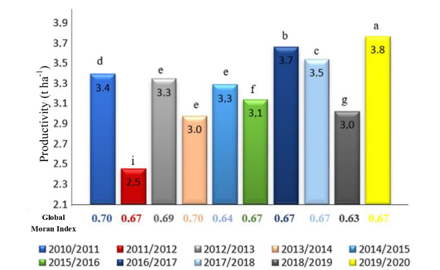
Fig. 1. Time distribution and Global Moran index of the mean soybean productivity in the state of Paraná; lowercase letters represent the comparison of mean productivity between harvest years (Z test, p<0.05), the same letters in mean values indicate that productivity is statistically equal.
the interval considered resulted in a mean reduction of 0.10 (t/ha) in mean productivity in the same VS. In turn, in relation to the indirect effect, a 1-mm increase in rainfall during the interval considered implied a mean reduction of 0.12 (t/ha) in mean productivity in all its neighboring VSs. Thus, in a general way, a 1-mm increase in rainfall during the interval was considered in a 0.22 (t/ha) reduction in mean productivity (Table 2).
The minimum temperature variable in the interval from the sowing date to 16 days before MVDD (SD_2a_MVDD) and the solar radiation variable in the interval from MVDD to CD (MVDD_CD, Table 2), which is the period of the year with the highest amount of solar radiation (Grzegozewski et al., 2017), had a similar behavior that of rainfall in the SD_MVDD_1b interval, which presented the lowest negative impact on mean productivity among the variables analyzed.
In the five municipalities in Paraná with the highest productivity values in the historical series studied (Cascavel, Guarapuava, Tibagi, Ponta Grossa, and Castro), the same behavior was observed in relation to the influence of climate and EV variables on soybean productivity.
For example, the municipality of Cascavel with the highest productivity values with 3.18 (t/ha), a 1mm increase in rainfall during the 1b_MVDD_CD interval, indicated by the total marginal effect (Table 2), imply a 0.62 (t/ha) increase. The same analysis can be performed for other municipalities and explanatory variables.
Discussion
Time analysis and spatial autocorrelation corresponding to soybean productivity
In this study, a soybean yield pattern was observed in different harvest years in the state of Paraná. Similar results were observed by Grzegozewski et al. (2020) and Silva et al. (2021), who evaluated the global spatial autocorrelation and spatial distribution of productivity in the state of Paraná in the harvest years from 2010/2011 to 2012/2013, using a spatial scale greater than \(9\ km\ \times \ 9\ km\). Thus, the study revealed greater precision in the mean soybean productivity pattern in the state.
In relation to the observed results (Table 1), Moran's global index corresponding to the explanatory variables showed higher values with the temperature variable. This was due to the regional homogeneity of the state. (Aparecido et al., 2016).
The variable EVI, which is the vegetation index, representing the good productive performance of soybeans (Trindade et al., 2019), in the interval of 8 days before to 8 days after the MVDD (1b_MVDD_1a; Table 1), presented the highest values in the 2019/2020 harvest year, which was the year with the highest productivity values (Figure 1).
Spatial panel data models
The Spatial Autoregressive (SAR) model with fixed effects best fitted the data to explain productivity as a function of the explanatory variables. This was verified using Lagrange and robust Lagrange tests, as well as by means of the AIC (Supplementary 1
Table 3).
Thus, the estimates of the direct, indirect, and total marginal effects corresponding to the dependent variables of the SAR model showed that rainfall (Rain_1b_MVDD_CD, Table 2) exerted a positive effect on productivity. According to Farias et al. (2007), this is because, in this period, which includes the grain's flowering and filling period, rainfall influences soybean development. In addition, the higher water consumption by the plant coincided with the period in which the crop presented more height and a higher leaf area index.
Table 2. Direct, indirect, and total effects of the SAR model, with fixed effects.
| Variables | Direct Effect |
Indirect Effect |
Total Effect |
|---|---|---|---|
| Rain_1b_MVDD_CD | 0.09* | 0.11* | 0.20* |
| Rain_SD_MVDD_1a | -0.10* | -0.12* | -0.22* |
| EVI_1b_MVDD_1a | 0.14* | 0.17* | 0.31* |
| EVI_SD_MVDD_2a | 0.21* | 0.24* | 0.45* |
| Tme_SD_2b_MVDD | 0.19* | 0.22* | 0.42* |
| Tmin_SD_2b_MVDD | -0.23* | -0.27* | -0.50* |
| Tmax_1b_MVDD_1a | -0.003NS | -0.01NS | -0.01NS |
| SR_MVDD_CD | -0.04* | -0.04* | -0.08* |
| ETp_MVDD_2a_CD | 0.01* | 0.01* | 0.02* |
*(p<0.05), NS: Not Significant.
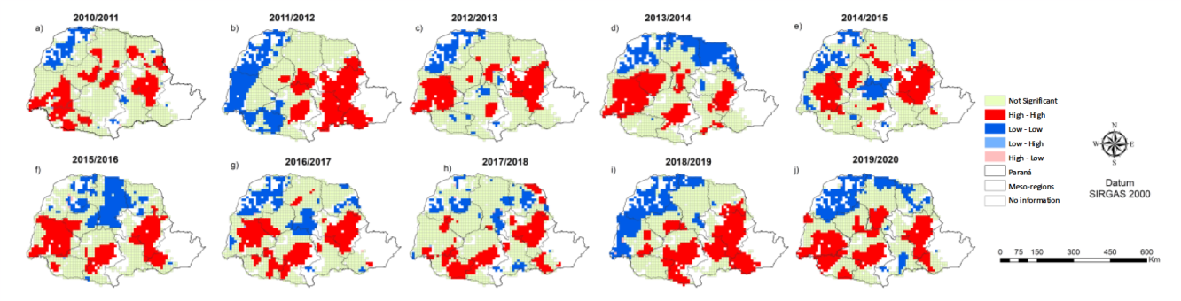
Fig. 2. Lisa Cluster Map corresponding to the “productivity” variable of the following harvest years: a) 2010/2011, b) 2011/2012, c) 2012/2013, d) 2013/2014, e) 2014/2015, f) 2015/2016, g) 2016/2017, h) 2017/2018, i) 2018/2019, and j) 2019/2020.

Fig 3. Study area in the state of Paraná; example of an ECMWF virtual station (EV) with the percentage of the area of 4 municipalities (a1, a2, a3, a4).
The EVI variable in the interval 1b_MVDD_1a (Table 2) had a positive impact on productivity, being the moment of the soybean phenological stages of flowering and pod formation (from R1 to R3), where in general, the highest EVI values were observed in the profile temporal spectral (Johann et al., 2016).
The mean temperature variable in the SD_2b_MVDD interval exerted a positive impact on productivity, as the ideal range for rapid and uniform emergence is close to 25°C (Farias et al., 2007), and the beginning of soybean sowing in the state is preferably in October of each harvest year (Johann et al., 2016) when temperatures are around this value.
In relation to potential evapotranspiration in the MVDD_2b_CD interval, the results showed little impact on mean productivity (Table 2), which can be justified because it is in these phenological stages that the smallest amounts of the crop's potential evapotranspiration are observed.
On the other hand, the accumulated rainfall variable in the SD_MVDD_1b interval exerted a negative impact on mean productivity. Excessive rainfall and cloudy days are believed to cause anomalies in plant development (Pereira et al., 2016). In addition, during germination, both excess and deficit water are detrimental to achieving uniformity in the number of plants per planted area (Silva et al., 2016).
In municipalities with the highest productivity values, rainfall between the sowing date and 16 days after MVDD (SD_MVDD_1a), almost 75% of this rainfall volume contributed to excellent productivity.
The productive performance of the crop can be translated by the variable EVI, which is a vegetation index that represents the vigor of the plant (Trindade et al., 2019), and was one of the highest values of marginal effects observed in this interval.
In relation to the mean and minimum temperature variables in the SD_2b_MVDD interval, rainfall during this period minimized the harmful effects of temperature (Birthal et al., 2014), as the ideal temperature for the period is around 25°C, to provide fast and uniform emergence (Garcia et al., 2007).
Materials and Methods
Study area
The study area selected was the state of Paraná located in southern Brazil, with a territorial area of 199,298.982 km², comprised of 399 municipalities (IBGE, 2022a), and with a Gross Domestic Product (GDP) of $USD 104 billion in 2021, which equals 6.67% of the Brazilian GDP during the period (IPARDES, 2021; Figure 3).
Soybean productivity and climate variables
The mean soybean yield data (t/ha) for the ten harvest years of the Paraná municipalities were obtained from the Brazilian Institute of Geography and Statistics (IBGE, 2022b).
Data corresponding to rainfall (mm), mean, minimum, and maximum air temperature (°C), and global solar radiation (MJ/m2/day) climate variables were obtained using the Google Earth Engine (GEE) web platform, from the European Center for Medium-Range Weather Forecast (ECMWF) model with virtual stations (VSs) offering a spatial resolution of \(9\ km \times 9\ km\) (ECMWF, 2021; GOOGLE LLC, 2021).
In addition to these variables, the potential evapotranspiration (mm) climate variable was also included (Embrapa, 2022). To acquire the data corresponding to this variable, GEE was used in the Colab running environment using Python. In addition, to determine the values of the productivity and potential evapotranspiration variables in the same VS locations, ArcGIS software version 10.3 (ESRI, 2018) was used.
Enhanced Vegetation Index (EVI) values were extracted from the Moderate Resolution Imaging Spectroradiometer (MODIS) sensor (Embrapa, 2022).
The EVI spectral-time profile was only considered in the places mapped with soybean crops using satellite images, avoiding the analysis in regions with no plantations.
For this purpose, the mappings performed for the following harvest years were considered: 2010/2011 and 2011/2012 (Souza et al., 2015); 2012/2013 and 2013/2014 (Grzegozewski et al., 2016), 2014/2015 and 2015/2016 (Verica, 2018); and 2016/2017, 2017/2018, 2018/2019, and 2019/2020 (Paludo et al., 2020). ArcGIS software, version 10.3 (ESRI, 2018) was used to determine the EVI values at the same VSs locations.
Timesat software was used from extracted the parameters Sowing Date (SD), Maximum Vegetative Development Date (MVDD), and Collection Date (CD) (Savitzky and Golay, 1964). Furthermore, those that lacked profile characteristics of soybeans were not considered in the dataset. In this way the panel database contains 16,990 observations.
Measures associated with the climate variables and of the Enhanced Vegetation Index
Variables considered as explanatory variables were generated in the modelling, associated, according to the soybean phenological phases. Being call variables are the measures associated with the climate variables (AMVs) and EVI, totalling 98 explanatory variables.
These measures were defined as follows. For rainfall, solar radiation, potential evapotranspiration, and EVI, the accumulated value in each interval was considered, whereas for the mean, minimum, and maximum temperatures, the mean of the interval was considered. In addition, the value was considered in the MVDD for all variables described in Supplementary 1 Figure 1.
Subsequently, we verified whether the explanatory variables exhibited multicollinearity. Multicollinearity imposes a high and imperfect correlation between two or more explanatory variables (Wooldridge, 2012). For this, the Variance Inflation Factor (VIF) measure was used for each explanatory variable, described in Supplementary 2 Equation (1); Marques et al., 2022).
After verifying the existence of multicollinearity, variables among the 98 AMVs were selected using the Non-Negative Garrote (NNG) method, as it presents the best results in papers related to the selection of variables in a panel data set, described in Supplementary 2 Equation (2); Vrigazova, 2017; Yuan and Lin, 2007).
Descriptive analysis and spatial autocorrelation
A descriptive analysis of the mean soybean productivity in each harvest year was performed, in addition to comparing it between harvest years via the Z test at 5% likelihood.
Subsequently, spatial analysis was performed using the Global Moran Index (\(I\)) described in Supplementary 2 Equation 4 (Almeida, 2012) to verify the characteristics of the spatial distribution of the variables under study in each harvest year. To calculate the Global Moran Index, it was verified whether the variable presented a likelihood normal distribution behavior by means of Jones test 5% significance (Jones, 1969). For those that did not present this pattern, the Box-Cox transformation was used (Box and Cox,1964).
The Queen spatial weighing matrix was used in this study, although the Torre matrix was tested, and the results were similar to Queen. Consequently, the choice was for the Queen matrix, as the same spatial weighing matrix should be used in all analyses (Almeida, 2012).
The values of I can be positive between 0 and 1, indicating the existence of a direct spatial correlation of a variable, that is, VSs with high values are surrounded by VSs with high values, with a sense analogous to low values of the same variable. In contrast, negative values of I between 0 and 1 indicate an inverse spatial autocorrelation, that is, VSs with high values have neighbors with low values, or vice versa (Anselin et al., 2005).
Panel data and spatial panel data model
Panel data, it is the combination of cross-section data with time series, described in Supplementary 1 Figure 2 (Gujarati and Porter, 2011). Before estimating the spatial model, it is necessary to verify whether it is appropriate to include unobserved effects when compared to the clustered data model described in Supplementary 1 Figure 3 Almeida (2012).
The presence of spatial dependence justifies using spatial panel data modeling. In this context, among the model they exist the Spatial Autoregressive (SAR) model and the Spatial Error Model (SEM) (Supplementary 1 Figure 3; Ortiz et al., 2022).
In the panel model estimates, a combination of two effects was used: individual and time (two-way). This is because, in this way, both the effects related to the units (VSs) and to time (harvest years) are considered.
After verifying the presence of spatial dependence, the following tests were applied to choose the best spatial model: the Lagrange multiplier test for spatial lag (LM lag), Lagrange multiplier test for the spatial error term (LM error), robust spatial lag Lagrange multiplier test (LM lag (robust)), and robust spatial error term Lagrange multiplier (LM error (robust)). A significance level of 5 % was used to perform the tests described in Supplementary 1 Figure 4 (Anselin et al., 2008).
In addition to using the Lagrange Multiplier tests to select the best spatial model, the Akaike Information Criterion (AIC) (Almeida, 2012).
After selecting the best model, the normality and homoscedasticity assumptions were verified in the residuals from the selected model. This verification of the assumptions becomes necessary to check the robustness of the parameters estimated by the regression models of panel data analyses, 5% significance level was used for both tests (Arruda et al., 2015).
The normality assumption was used to determine whether the error of the model presented a normal distribution. One way to verify normality is to use the Jarque-Bera test (Gujarati and Porter, 2011). However, based on the Central Limit Theorem, and given the high number of observations, this assumption can be waived (Arruda et al., 2015). To verify whether the distribution of the residuals was homoscedastic, the Breusch-Pagan test was used (Coscarelli et al., 2011).
One of the main interests of regional scientific studies is to verify the impact of changing a certain VS in the neighborhood. For this, the concepts of direct and indirect effects are used. That is, the direct effect measures the change in the impact of an explanatory variable of a given VS, in relation to the dependent variable of that same VSs. On the other hand, if there are changes not only in the dependent variable in that VS, but also in the dependent variable in other VSs the indirect effect (Elhorst, 2014).
The local indirect effect is the impact of a given region on its closest neighbors, defined through the connectivity of the weight matrix. In our study, we used the Queen weight matrix (Guliyev, 2020).
Thus, when considering a given virtual station, called the system origin virtual station (VS1), what happens in VS1\({EV}_{1}\) exerts a local indirect effect on the neighboring VSs, determined by the connectivity defined by the Queen weight matrix (VS2 to VS9; Supplementary 1 Figure 5). In turn, the global indirect effect consists of the overflow of what happens in a given VS to all other VSs surveyed.
A phenomenon that occurs in overflow is called feedback, which is a characteristic of the spatial regression model and arises as a result of impacts between neighboring units (Lesage and Pace, 2009). This can be seen in Supplementary 1 Figure 5 between VS4 and VS5 (indicated by the red arrow); that is, the impact that VS4 exerted on VS5 ends up returning to itself. With the expansion of this behavior among several VSs, a simultaneous feedback effect occurs; that is, all VSs both exert an impact and are impacted (Lesage, 2008).
The intensity of the feedback depends on the position of the VS in space, the degree of connectivity between the VSs determined by the weight matrix, the spatial dependence degree, and the estimated values of the \(\widehat{\beta}\) coefficients associated with the explanatory variables (Lesage, 2008).
One of the advantages of estimating the SAR spatial lag model is the possibility of quantifying overflow effects through measurements of the following marginal effects: direct, indirect and total (Souza et al., 2021).
Thus, for the SAR model, the direct and indirect effect measures were calculated through the partial derivatives of the expected value of the SAR model dependent variable in relation to each explanatory variable. This calculation will result in matrix \(\mathbf{S}_{k}\left( \mathbf{W} \right) = {{(\mathbf{I}}_{n}\ - \ \ \rho\mathbf{\ }\mathbf{W}\mathbf{)}}^{- 1}{\mathbf{I}_{n}\beta}_{k}\) sized \(n \times n\), where \(\mathbf{I}_{n}\) is an identity matrix (\(n \times n\)); \(\mathbf{W}\) is the spatial weight and positive matrix sized \(n \times n;\ \) since in this research the Queen spatial weight matrix was used; \(\rho\) is the spatial dependence coefficient; and \(\beta_{k}\) is the coefficient associated with the \(k\)-th explanatory variable (Lesage and Pace, 2009).
Thus, the direct marginal effect in relation to the \(k\)-th explanatory variable (\(k = 1,\ldots p\)) corresponds to the mean of the elements on the main diagonal (\({(s_{k}(\mathbf{W})}_{ii}\)) of matrix \(\mathbf{S}_{k}\left( \mathbf{W} \right)\) where \(i = 1,\ \ldots,\ n\). On the other hand, the indirect marginal effect measure in relation to the \(k\)-th explanatory variable (\(k = 1,\ldots p\)) corresponds to the mean of the elements off the main diagonal (\({(s_{k}(\mathbf{W})}_{ij}\)) of matrix \(\mathbf{S}_{k}\left( \mathbf{W} \right)\), with \(i,j = 1,\ \ldots,\ n\) and \(i \neq j.\)
Furthermore, it was defined a climatological profile was outlined for the five municipalities in Paraná, which were the largest soybean producers in the state in the time series analyzed, representing approximately 7% of the state's productivity in each harvest year, namely Cascavel, Guarapuava, Tibagi, and Ponta Grossa.
Thus, an exploratory analysis of the rainfall and mean and minimum temperature explanatory variables was conducted in these municipalities. These variables were selected because they are the climatological variables with the greatest determining factor for the explanation of agricultural productivity in the panel data spatial model.
Selection of the variables, analyses of the models in panel data, and statistical tests were performed using the following R software packages: glmnet, nnGarrote, car, plm, plmtest, phtest, slmtest, spdep and pspatreg (R DEVELOPMENT CORE TEAM, 2022).
Conclusions
In all crop years analyzed, the spatial autocorrelation of productivity showed positive and significant values, indicating that productivity in virtual stations (EVs) with higher or lower soybean yields is surrounded by EVs with the same characteristics. The results revealed that the Spatial Autoregressive model with fixed effects was the most suitable model for analyzing variables in studies. The spatial parameters of the model and the Moran index indicated that changes in the productivity of a given VS affect the productivity of neighboring VSs. Furthermore, the estimates generated from the marginal effects of the SAR model revealed that, from 2010/2011 to 2019/2020, soybean productivity was positively related to precipitation in the interval 1b_MVDD_CD, with EVI, with the average temperature in the interval SD_2b_MVDD, and potential evapotranspiration in the MVDD_2a_CD interval. However, it was negatively related to precipitation in the SD_MVDD_1a interval, minimum temperature in the SD_2b_MVDD interval and solar radiation in the MVDD_CD interval. This was also observed in municipalities with higher soybean productivity. Based on the results obtained, it is possible for the gardener to diagnose the appropriate area for planting the crop, in relation to the impacts of climate variations and optimize decision-making about soybean cultivation.
Acknowledgments
The authors would like to acknowledge the Applied Statistics Laboratory (LEA) members of the Western Paraná State University (UNIOESTE) - Cascavel - Paraná - Brazil.
Almeida E (2012) Econometria Espacial Aplicada. Campinas, São Paulo, Brazil: Alínea.
Anselin L, Gallo JL, Jayet H (2008) Spatial panel econometrics. In: The econometrics of panel data: Fundamentals and recent developments in theory and practice. Berlin, Heidelberg: Springer Berlin Heidelberg.
Anselin L, Syabri I, Kho Y (2005) GeoDa: An introduction to spatial data analysis. Geogr Anal. 38(1):5-22.
Aparecido LO, Rolim S, Richetti J, Souza OS, Johann JA (2016) Köppen, Thornthwaite and Camargo climate classifications for climatic zoning in the State of Paraná, Brazil. Ciênc Agrotec. 40:405-417.
Arruda MP, Vieira CAM, Paulo E, Lucena WGL (2015) Análise do conservadorismo e persistência dos resultados contábeis das instituições financeiras brasileiras. SCG. 10 (2):23-35.
irthal PS Negi DS, Kumar S, Aggarwal S, Suresh A, Khan MT (2014) How sensitive is Indian agriculture to climate change? Indian J Agric Econ. 69 (4):474-487.
Blanc E, Reilly J (2017) Approaches to Assessing Climate Change Impacts on Agriculture: Na Overview of the Debate. Rev Environ Econ Policy. 11(2):247-257.
Box G, Cox D (1964) An analysis of transformations. Journal of the Royal Statistical Society Series B: J R Stat Soc Ser B Stat Methodol. 26(2):211-252.
Corrêa ABN, Marçal RR, Flach L (2019) Previsibilidade no Mercado de criptomoedas: Uma Modelagem Autorregressiva com Dados em Painel do Market Cap. RCGC. 2(1):51-62.
Coscarelli BV, Lamounier WM, Amaral HF (2011) Liquidez corporativa e o market value added. Adv Sci Appl Account. 4(3):304-330.
ECMWF - European Centre for Medium-Range Weather Forecasts. 2021. ERA5-Land hourly data from 1950 to presente. https://cds.climate.copernicus.eu/cdsapp#!/dataset/reanalysis-era5-land?tab=form.
lhorst JP (2014) Spatial Econometrics from Cross-Sectional Data to Spatial Panels. New York: Springer.
EMBRAPA - EMPRESA BRASILEIRA DE PESQUISA AGROPECUÁRIA (2022) Banco de produto MODIS: Base estadual brasileira https://www.modis.cnptia.embrapa.br/geonetwork/srv/pt/main.home.
ESRI (2018) ArcGIS for Windows Version 10.3. License type ArcInfo. ESRI - Enviromental Systems Research Institute.
Farias JRB, Nepomuceno AL, Neumaier N (2007) Ecofisiologia da Soja, Circular Técnica, Londrina, Brazil: Embrapa Soja. 48(1):1-9.
Garcia A, Pípolo AE, Lopes ION, Portugal FAF (2007) Instalação da lavoura de soja: época, cultivares, espaçamento e população de plantas, Circular Técnica, Londrina, Brazil: Embrapa Soja. 51:1-12.
GOOGLE LLC - GOOGLE EARTH ENGINE - GEE (2021) https://earthengine.google.com.
Grzegozewski DM, Cima EG, Uribe-Opazo, MA, Guedes LPC, Johann AJ (2020) Spatial and Multivariate Analysis of Soybean Yield in the State of Paraná-Brazil. J Agric Res. 8(1):387-412.
Grzegozewski DM, Johann JA, Uribe-Opazo MA, Mercante E, Coutinho AC (2016) Mapping soya bean and corn crops in the State of Paraná, Brazil, using EVI images from the MODIS sensor. Int J Remote Sens. 37(1):1257-1275.
Grzegozewski DM, Uribe-Opazo MA, Johann AJ, Guedes LPC (2017) Spatial correlation of soybean productivity, enhanced v vegetation index (EVI) and agrometeorological variables. Eng Agríc. 37(3):541-555.
Gujarati DN, Porter DC (2011) Econometria Básica, 5th Edn. PortoAlegre, Brazil: AMGH.
Guliyev H (2020) Determining the spatial effects of COVID-19 using the spatial panel data model. Spat Stat. 38(1):100443
Hirakuri MH (2021) Perdas econômicas geradas por estresses bióticos e abióticos na produção brasileira de soja no período 2016-2020. Londrina, Brazil: Embrapa.
IBGE - Instituto Brasileiro de Geografia e Estatística (2022a) Brasil em Síntese. https://cidades.ibge.gov.br/brasil/pr/panorama
IBGE - Instituto Brasileiro de Geografia e Estatística (2022b) Banco de dados agregados. https://sidra.ibge.gov.br/tabela/1612.
IPARDES – Instituto Paranaense de Desenvolvimento Econômico e Social (2021) PIB do Paraná - Resultados do 4⁰ Trimestre de 2021.
Johann JA, Becker WR, Uribe-Opazo MA, Mercante E (2016) Estimating soybean development stages in Paraná state - Brazil through orbital modis images. Eng Agríc. 36(1):126–42.
Jones TA (1969) Skewness and kurtosis as criteria of normality in observed frequency distribuitions. J Sediment Res. 39(1):1622-1627.
Lesage JP (2008) An introduction to spatial econometrics. Rev Econ Ind. 123(3):19–44.
Lesage JP, Pace RK (2009) Introduction to Spatial Econometrics. Londres: CRC Press.
arques HR, Ávila ES, Zambalde AL, Pereira RM (2022) Inovação Aberta e Implementação de Diferentes tipos de Inovação: Uma Análise Baseada em Dados em Painel. Bras Bus Ver. 19(1):40-58.
Nadine S, Ntsama E (2022) Does Human Capital Influence Agricultural Production? A Case Study on Cereals Production in the Cemac Zone. Int J Food Agric Econ. 10(2): 131–141.
Nitsche PR, Caramori PR, Ricce WS, Pinto LFD (2019) Atlas climático do estado do Paraná. Londrina, Paraná, Brazil: Instituto Agronômico do Paraná.
Ortiz CRA, Méndez P, Flores-Chamba J (2022) Environmental impact of the shadow economy, globalisation, and human capital: Capturing spillovers effects using spatial panel data approach. J Environ Manage. 308(1):114663.
Paludo A, Becker WR, Richetti J, Silva LCDA, Johann JA (2020) Mapping summer soybean and corn with remote sensing on Google Earth Engine cloud computing in Parana state – Brazil. Int J Digit Earth.13(12):1624-1636.
Pereira CS, Serafim RC, Zanatto IB, Fiorini IV (2016) Germinação e crescimento inicial de plantas de soja submetidas ao déficit hídrico. Glob Educ J Sci Tecnol. 9 (1):33-40.
R Development Core Team (2022) R: a language and environment for statistical computing. Vienna, Austria: R Foundation for Statistical Computing. URL http://www.R-project.org
Savitzky A, Golay MJE (1964) Smoothing and differentiation of data by simplified least squares procedures. Anal Chem. 36(2):1627-1639.
Silva EM, Gasparin PG, Paludo A, Becker WR, Guedes LPC, Johann JA (2021) Soybean Productivity and Agrometeorological Variables Assessed from the perspective of Spatial and Circular Statistics. J Agric Stud. 9(3):303-325.
Silva M, Sibaldelli R, Neumaier N, Mertz-Henning LM, Nepomuceno A, Farias J (2016) Análise da disponibilidade hídrica nas safras 2014/15 e 2015/16. Londrina, Brazil: Embrapa Soja, 11(1): 68-74.
Souza CHW, Mercante E, Johann JA, Lamparelli RAC, Uribe-Opazo MA (2015) Mapping and discrimination of soya bean and corn crops using spectro-temporal profiles of vegetation indices. Int J Remote Sens, 36(7):809-1824.
Souza HG, Costa EM, Tabosa FJS, Castelar PUC (2021) Climate Sensitivity and the Value of Agricultural Production in the Brazilian Northeast: An Approach Using Spatial Panel Data. Int J Bus Adm. 12(5):1-20.
Tan Q, Liu Y, Dai L, Pan T (2021) Shortened key growth periods of soybean observed in China under climate chang. Sci Rep.11(1):8197.
Trindade FC, Alves MC, Noetzold R, Andrade IC, Pozz, AAA (2019) Relação espectro-temporal de índices de vegetação com atributos do solo e produtividade da soja. Bras Cienc Agrar. 62(1):1-11.
Verica WR (2018) Mapeamento semiautomático por meio de padrão espectro-temporal de áreas agrícolas e alvos permanentes com EVI/MODIS no Paraná. Master’s dissertation - Universidade Estadual Oeste do Paraná, Cascavel, Paraná, Brazil.
Vrigazova BT (2017) Property rights: Factors Contributing to the Generation of Income from Ownership of Property. Innov Model Anal J Res. 2(1):22-39. Wooldridge JM (2012) Introductory Econometrics: A Modern Approach, 5th edn. Canadá: Cengage Learning.
Yuan M, Lin Y (2007). On the non-negative garrotte estimator. J R Stat Soc Ser B Methodol. 69(2):143-161.
Yuzbashkendi SS (2019) Climate and Government’S Guaranteed Price Policy Effects on the major oilseed’s cultivation area and land rental in Iran. Int J. Food Agric Econ. 7 (3) 257 - 269.