
Aust J Crop Sci. 19(01):44-51 (2025) | ISSN:1835-2707
https://doi.org/10.21475/ajcs.25.19.01.p169
Spatial variability of soybean productivity and soil attributes: "hole effect" and local diagnosis with the Wave model
Amilton Luciano Garcia da Silva¹*, Miguel Angel Uribe-Opazo¹, Gustavo Henrique Dalposso², Luciana Pagliosa Carvalho Guedes¹
¹Western Paraná State University – (UNIOESTE), Cascavel, Paraná, Brazil²Federal University of Technology Paraná – (UTFPR), Toledo, Paraná, Brazil
*Corresponding author: Amilton Luciano Garcia da
Silva 
Abstract: Soybean is one of the most important commodities on a global scale. Therefore, studies in precision agriculture (PA) are essential to maximize economic return and minimize environmental impacts. In this context, conducting interpolations to map soybean productivity and soil attributes plays a crucial role on decision-making and should represent an efficient estimate of actual field conditions. In this situation, the study employed the geostatistical Wave model to assess local influences on several response variables, including soybean productivity, soil resistance to penetration, copper content, and soil pH. The model accounts for spatial dependence in the data, particularly when the semivariance exhibits the ‘hole effect’. Techniques for diagnosing local influence were developed for spatial data using the Wave model and the results showed that the identification and removal of influential observations caused relevant changes in the estimates of parameters that define the structure of spatial dependence, directly impacting the construction of interpolated maps. This interferes with the creation of differentiated management zones, considering profitability and soil attributes. These findings highlight the importance of considering local influence when analyzing spatial data to ensure the accuracy of the results obtained.
Keywords: geostatistics; kriging; local influence diagnosis; maximum likelihood; productivity map, spatial data analysis, spatial statistics.
Abbreviations: AIC_Akaike Information Criterion; BIC_Bayesian Information Criterion; Cu_soil copper content; Cu#36_copper without the influential observation #36; ML_maximum likelihood; PA_precision agriculture; pH_soil pH; pH#99_soil pH without the influential observation #99; Prod_soybean productivity; Prod#85_soybean productivity without the influential observation #85; \(RSP_{0.21 - 0.30m}\)_soil penetration resistance at a depth of 0.21 to 0.30 meters depth layer; \(RSP_{0.21 - 0.30m}\)#46_soil penetration resistance in the 0.21 to 0.30 meters depth layer without the influential observation #46; SDI_Spatial Dependency Index.
Introduction
Precision agriculture is an innovative approach aimed at optimizing agricultural crop management, taking into account the spatial and/or temporal variability of factors affecting production. This approach brings various potential benefits, such as improvement in crop quality, reduction of environmental impact, increased sustainability, ensuring food security, promoting economic development, and enhancing profitability and productivity (Zain et al., 2024).
To implement precision agriculture, it is necessary to use methods that allow for describing and modeling the spatial variability of natural phenomena, as well as estimating values at unsampled locations. Among the existing methods in precision agriculture studies, geostatistics stands out, offering adaptations of classical statistical techniques to take advantage of the special dependence present in the data to generate interpolated maps (Uribe-Opazo et al., 2023, Lorbieski et al., 2023). In this context, kriging is a geostatistical interpolation method, defined by Isaaks and Srivastava (1989) as the best spatial linear interpolator with minimum variance.
Kriging requires fitting theoretical models to the experimental semivariogram, which is a function that measures the degree of spatial dependence of a georeferenced variable (Uribe-Opazo et al., 2012). The most common models used in geostatistics are the Exponential, Spherical, Gaussian, and Matérn family models (Cressie, 2015). These models are monotonic and increasing, meaning they continuously increase with the distance between points.
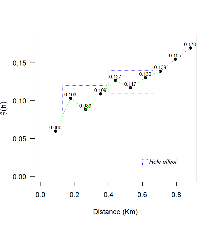
However, in some cases, the semivariogram may exhibit non-monotonic behavior, meaning it does not continuously increase with distance, indicating high values surrounded by low values, generating a sinusoidal movement of the semivariance function, known as the "hole effect". For these cases, Wave model is the most suitable, as it can more effectively handle the non-monotonic variation of the semivariogram (Carvalho et al., 2009; Dalposso et al., 2022).
According to Dalposso et al. (2022), neglecting these non-monotonic structures in the analysis can lead to erroneous interpretations, as the adopted model may not reproduce the observed patterns of spatial variability. Additionally, the presence of influential observations can significantly alter the results of spatial dependence analyses and, consequently, the construction of maps generated by kriging.
To assess whether observations can cause distortions in spatial dependence models, Cook (1986) proposed inducing small perturbations in the model or data. This technique, known in the literature as local influence, takes into account geometric differentiation and deviation from likelihood, which was employed as a procedure to evaluate the influence of observations (Uribe-Opazo et al., 2012; De Bastiani et al., 2015).
Precision agriculture has benefited from various studies on local influence analysis, as proposed by De Bastiani et al. (2015), Dalposso et al. (2021) and Uribe-Opazo et al. (2021, 2023). These studies contribute to advancing knowledge in the field. However, there are still no works addressing the diagnosis of local influence in the context of the Wave geostatistical model.
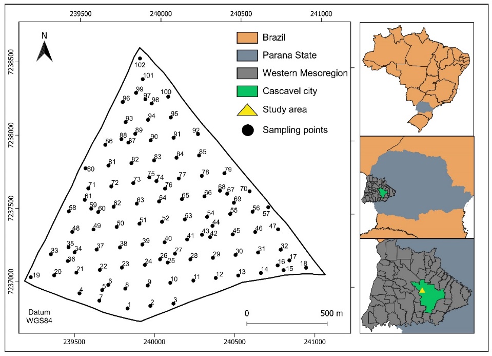
Fig 1. Location of the 102 sampling points.
In this context, this study aimed to develop and apply techniques for diagnosing local influence on the response variable when employing the Wave model to describe the spatial variability of soybean productivity, crucial for crop profitability; soil copper content, influencing plant growth; soil pH, affecting nutrient availability; and soil penetration resistance, impacting root development. The local influence diagnosis techniques allowed for identifying influential observations on the response variable, highlighting observations that may affect parameter estimates, model-predicted values, and the construction of maps through kriging
Results and discussion
Exploratory analysis
Table 1 displays the descriptive statistics of the variables: soybean productivity (Prod [\(t\ ha^{- 1}\)]), soil copper content (Cu [\(mg\ dm^{- 3}\)]), soil pH (pH) and soil penetration resistance at a depth of 0.21 to 0.30 m (\(RSP_{0.21 - 0.30m}\) [MPa]). During the 2022/2023 growing season, the average soybean productivity in the monitored area was 1.533 \(t\ ha^{- 1}\), considered low compared to the state's productivity (3.860 \(t\ ha^{- 1}\)) and national (3.507 \(t\ ha^{- 1}\)) in the same period (Conab, 2023). These results are lower than those found by Dalposso et al. (2021) who conducted studies on soybean productivity in the same city where the experiment was carried out.
The results also indicate that the average soil copper content was classified as low (0.69 \(mg\ dm^{- 3}\)) according to Santos and Silva (2001). Conversely, the average pH value (5.82) was considered high by the same authors. This result is higher than that found by Dalposso et al. (2018), who conducted experiments on soil pH content in the same city where the study was conducted. Regarding \(RSP_{0.21 - 0.30m}\), the average was 2.19 MPa, indicating a low level of soil compaction, with little limitation on root development, according to Canarache's criteria (1990).
Soybean productivity and soil copper content showed the highest coefficient of variation, indicating heterogeneity (CV ≥ 30%). Similar results were found by Maltauro et al. (2023), who conducted a trial in the same region where this research was carried out. None of the variables under study presented outliers.
The spatial distribution of the sample values was analyzed using a post-plot chart, presented in Figure 2. This chart allows for checking the presence of clustering and directional trends of high or low sample values.
Figure 2(a) shows that, overall, the highest soybean productivity values (\(t\ ha^{- 1}\)) are located in the central and southern regions of the monitored area. Conversely the northern and central regions
predominantly present samples in the two lower classes of the chart (minimum value up to the median), indicating a region of lower productivity. Figure 2(b) reveals that the highest copper values are concentrated in the southwest region, which stands out as the richest in this nutrient. Figure 2(c) indicates that the lowest pH values are concentrated in the northern and southeastern regions, characterizing more acidic soil. Figure 2(d) indicates that the highest values of \(RSP_{0.21 - 0.30m}\) are located in the central and northern regions, suggesting greater limitation to root growth.
Variographic analysis
For the spatial dependence analysis, 11 lags up to a distance of 880 meters (50% cutoff point) were considered (Clark, 1979). The semivariogram was examined in directions 0º, 45º, 90º, and 135º and confirmed that the data are isotropic (Guedes et al., 2013).
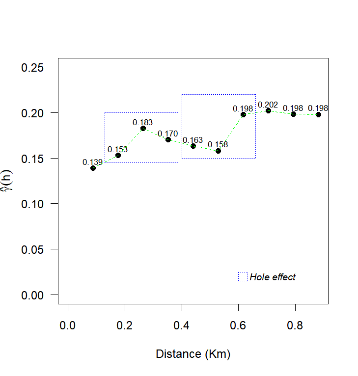
The analysis of the experimental semivariogram revealed an oscillatory behavior of the semivariances, characterized by alternating increases and decreases. This pattern has been reported in other studies on precision agriculture (Santra et al., 2008; Amirinejad et al., 2011; Dalposso et al., 2022) and was best fitted by the Wave model. This model is suitable for data with periodicity, which generate a "hole effect" due to positive and negative correlations between distant regions (Mahdi et al., 2020). The maximum likelihood method was used to estimate the parameters of the spatial dependence structures observed in Figure 3. The fitted models included Exponential, Gaussian, Matérn family with smoothing parameters k = 0.7, 1.0, and 2.0 as well as the Wave model.
Utilizing cross-validation criteria (Faraco et al., 2008), the Akaike Information Criterion - AIC (Akaike, 1973), and the Bayesian Information Criterion - BIC (Schwarz, 1978), the Wave model demonstrated the best performance for all the variables under study (Prod [\(t\ ha^{- 1}\)], Cu [\(mg\ dm^{- 3}\)], pH, \(RSP_{0.21 - 0.30m}\) [MPa]) (Table 2).
Based on the results of the Spatial Dependency Index - SDI (Table 2), it is evident that soybean productivity is associated with strong spatial dependence among the observations (SDI > 24%). Additionally, a relationship of moderate spatial dependence among the observations for copper is observed, pH and \(RSP_{0.21 - 0.30m}\) (11% < SDI ≤ 24%).
These results highlight the influence of the spatial distribution of these variables on agronomic characteristics and soybean crop productivity, providing valuable insights for understanding variability patterns in the growing environment.
Based on ordinary kriging interpolation and information from the Wave model, which best fit the semivariance function for all
| Table 1. Descriptive analysis of response and explanatory variables. | ||||
|---|---|---|---|---|
| Statistics | Prod | Cu | pH | RSP(0.21-0.30m) |
| Minimum | 0.330 | 0 | 4.60 | 1.23 |
| \(1^{st}\) Quartile | 1.045 | 0.38 | 5.50 | 1.89 |
| Median | 1.442 | 0.68 | 5.90 | 2.22 |
| Mean | 1.533 | 0.69 | 5.82 | 2.19 |
| \(3^{rd}\) Quartile | 1.988 | 1.02 | 6.20 | 2.47 |
| Maximum | 2.909 | 1.73 | 6.70 | 2.96 |
| SD | 0.607 | 0.43 | 0.43 | 0.38 |
| CV (%) | 39.59 | 62.69 | 7.40 | 17.39 |
| \[{\widetilde{u}}_{3}\] | 0.38 | 0.21 | -0.49 | -0.20 |
| Kur | -0.69 | -0.84 | 0.04 | -0.77 |
| SD: standard desviation; CV: coefficient of variation; \({\widetilde{u}}_{3}\): coefficient of skewness; Kur: coefficient of kurtosis; Prod: soybean productivity in the 2022/2023 crop year; Cu: copper; \(RSP_{0.21 - 0.30m}\): soil penetration resistance in the 0.21 to 0.30 meters depth layer. | ||||
| Table 2. Parameters estimates by maximum likelihood and asymptotic standard errors in parenthesis. | ||||||||
|---|---|---|---|---|---|---|---|---|
| Prod | Prod#85 | Cu | Cu#36 | pH | pH#99 | RSP 0.21-0.30m |
RSP 0.21-0.30m #46 |
|
| \[\widehat{\mu}\] | 1.794 (0.356) |
1.777 (0.355) |
0.686 (0.080) |
0.687 (0.081) |
5.837 (0.049) |
5.846 (0.062) |
2.198 (0.113) |
2.195 (0.113) |
| \[{\widehat{\varphi}}_{1}\] | 0.229 (0.191) |
0.229 (0.204) |
0.117 (0.040) |
0.118 (0.040) |
0.109 (0.028) |
0.154 (0.028) |
0.095 (0.034) |
0.096 (0.034) |
| \[{\widehat{\varphi}}_{2}\] | 0.481 (0.391) |
0.501 (0.402) |
0.061 (0.033) |
0.061 (0.033) |
0.077 (0.029) |
0.030 (0.021) |
0.049 (0.039) |
0.048 (0.039) |
| \[{\widehat{\varphi}}_{3}\] | 0.489 (0.135) |
0.476 (0.127) |
0.166 (0.024) |
0.166 (0.024) |
0.068 (0.004) |
0.146 (0.031) |
0.357 (0.111) |
0.354 (0.110) |
| \[\widehat{a}(km)\] | 1.462 | 1.424 | 0.498 | 0.497 | 0.610 | 0.438 | 1.068 | 1.060 |
| \[SDI\] | 39.90 | 40.42 | 11.38 | 11.36 | 16.84 | 4.76 | 20.04 | 19.83 |
| \[Class\] | strong | strong | moderate | moderate | moderate | weak | moderate | moderate |
| \(\widehat{\mu}\): mean; \({\widehat{\varphi}}_{1}\): nugget; \({\widehat{\varphi}}_{2}\): sill; \({\widehat{\varphi}}_{3}\): function range; \(\widehat{a}\): range; \(SDI\): spatial dependence index; \(Class\): classification; Prod: soybean productivity with all observations; Prod#85: soybean productivity without the influential observation #85; Cu: copper with all observations; Cu#36: copper without the influential observation #36; pH#99: pH without the influential observation #99; \(RSP_{0.21 - 0.30m}\): soil penetration resistance in the 0.21 to 0.30 meters depth layer with all observations; \(RSP_{0.21 - 0.30m}\)#46: soil penetration resistance in the 0.21 to 0.30 meters depth layer without the influential observation #46. | ||||||||
the variables under study, a soybean productivity map was generated (\(t\ ha^{- 1}\)), of copper content (\(mg\ dm^{- 3}\)), of soil pH and \(RSP_{0.21 - 0.30m}\) (MPa) (Figure 4).
Local influence diagnosis
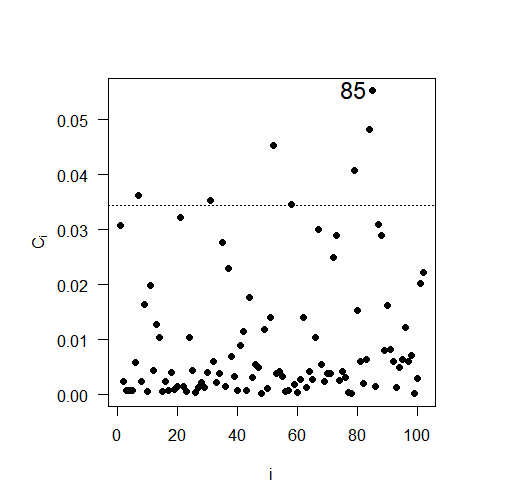
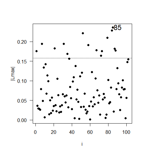
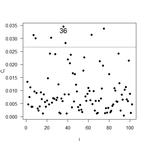
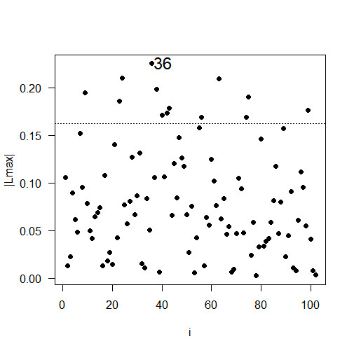
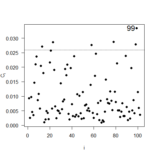
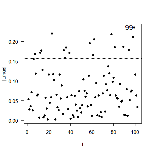
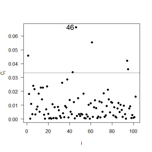
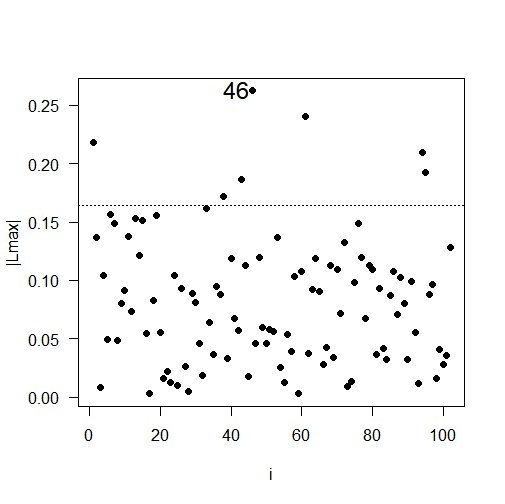
The objective of this section was to verify whether observations might be exerting local influence on the likelihood deviation, using local influence diagnosis techniques, employing the \(C_{i}\) and |\(L_{\max}\)| charts as a function of the order of observations (Cook, 1986). The local influence study was conducted for all the variables under study, using the perturbation scheme proposed by De Bastiani et al. (2015).
The results of the local influence analysis, illustrated in Figure 5, reveal the observations that have a significant influence on the likelihood deviation. The influential observations are: #85 for soybean productivity; #36 for soil copper content; #99 for soil pH; and #46 for soil penetration resistance.
As highlighted by Leiva et al. (2020) and Uribe-Opazo et al. (2023), it is important to note that in spatial statistics, an influential point is not necessarily an outlier, and vice versa. This distinction underscores the complexity of spatial relationships and the need to carefully consider the influence of individual points on the analysis results.
To assess the effect of influential observations on the analysis of spatial dependence structure and thematic map generation, the influential observations were excluded from the database for each variable, followed by a new analysis of spatial variability. This methodological approach allows for a deeper understanding of the spatial distribution of variables, adequately considering the influence of individual observations on the analysis results.
Considering this new context, without the presence of influential observations, the results are detailed in Table 2. According to cross-validation criteria (Faraco et al., 2008), the Akaike Information Criterion - AIC (Akaike, 1973), and the Bayesian Information Criterion - BIC (Schwarz, 1978), for soybean productivity without observation #85 (Prod#85), the Wave model, remains as the selected model to describe the spatial variability presenting similar values for the asymptotic standard errors.
Additionally, there is a reduction in the spatial dependence range by 38 meters, while still maintaining a strong spatial dependence according to the Spatial Dependency Index – SDI.
Likewise, for the other variables under study, without the influential observations, the selected model to describe the spatial variability continues to be the Wave model. However, changes are observed in the parameters estimated by the model. In the case of copper without observation #36 (Cu#36), the values are similar for the asymptotic standard errors and for the range. With regard to pH without observation #99 (pH#99), there was a substantial reduction of 172 meters in the spatial dependence range, resulting in a transition from moderate to weak classification according to the Spatial Dependence Index - SDI.
Finally, for the \(RSP_{0.21 - 0.30m}\) without observation #46 (\(RSP_{0.21 - 0.30m}\)#46), a reduction in the spatial dependence radius was observed by 8 meters, maintaining a moderate spatial dependence according to the Spatial Dependence Index – SDI.
Geostatistical map
When comparing the maps with all the observations (Figure 4 (a)) to those without the observation considered influential (Figure 4 (b)), it was observed that the spatial distribution of soybean productivity in the 2022/2023 growing season was similar, as indicated by the Kappa and weighted Kappa accuracy indices (Table 4) (\({\widehat{K}}_{w} \geq 0.75\)).
The comparative analysis between the thematic map of copper (Cu) considering all sample points (Figure 4 (c)) and the map excluding the influential observation #36 (Cu#36) (Figure 4 (d))

Fig 2. Post plot: (a) soybean productivity (\(\text{t\ }\text{ha}^{- 1}\)), (b) Copper (\(mg\ dm^{- 3}\)), (c) pH, (d) soil penetration resistance (MPa) in the layer 0.21 to 0.30 meters deep.
(a)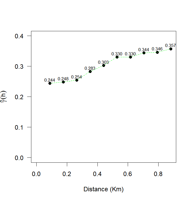 |
(b)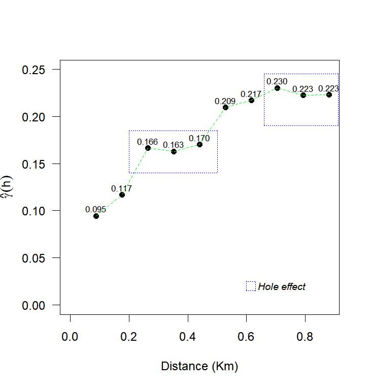 |
|---|---|
 |
 |
| (c) | (d) |
Fig 3. Experimental semivariance: (a) soybean productivity, (b) Copper, (c) pH, (d) soil penetration resistance in the layer 0.21 to 0.30 meters deep.
reveals similarity in the spatial distribution of copper values in the study area.
Copper is an essential element in the plants’ reproductive phase and consequently in determining crop productivity and quality, as well as being important for soybean resistance to diseases (Hansch and Mendel, 2009). In this sense, it is crucial to ensure a more efficient analysis of spatial variability so that plants receive an adequate amount of copper in their nutritional diet for sustainable development and satisfactory agricultural production.
When comparing the pH maps, both considering all the points (Figure 4 (e)) and excluding observation #99 99 (pH#99) (Figure 4 (f))), considered influential, significant differences were identified in the study areas. There is a decrease in the area corresponding to the upper end of the pH class, ranging from 6.10 to 6.31. The main change is the extinction of the area associated with the most acidic soils, with values below 5.45, according to the classification of Santos e Silva (2001).
According to Fagundes et al. (2018), for soybean cultivation, it is important that soil pH remains within the ideal range from 5.7 to 7.0 to ensure good plant development and satisfactory production. It is worth noting that soil pH is influenced by
various factors, such as fertilizer addition, the presence of organic matter, and soil type. In this sense, it is crucial to monitor and adjust soil pH to ensure adequate plant nutrition and high agricultural productivity.
When comparing the two maps for the \(RSP_{0.21 - 0.30m}\), study, Figure 4 (g) with all observations and Figure 4 (h) without the influential observation #46 (\(RSP_{0.21 - 0.30m}\)#46), it is noted similarity in the spatial distribution of \(RSP_{0.21 - 0.30m}\) values in the study area.
Soil compaction is a phenomenon that occurs when an external force is applied to the soil surface, altering its structure and properties (Keller et al., 2019; Vanderhasselt et al., 2023). In this study, it was found that the area most affected by soil compaction was the northern region of the property, where the terrain has a slight slope. This region also experiences higher machinery traffic, especially during turnaround maneuvers, increasing pressure on the soil.
Map comparison
The use of estimates of the Kappa (\(\widehat{K}\)) and weighted Kappa (\({\widehat{K}}_{w}\)) accuracy indices provides a non-subjective approach for the comparative analysis of maps, allowing for the quantification of
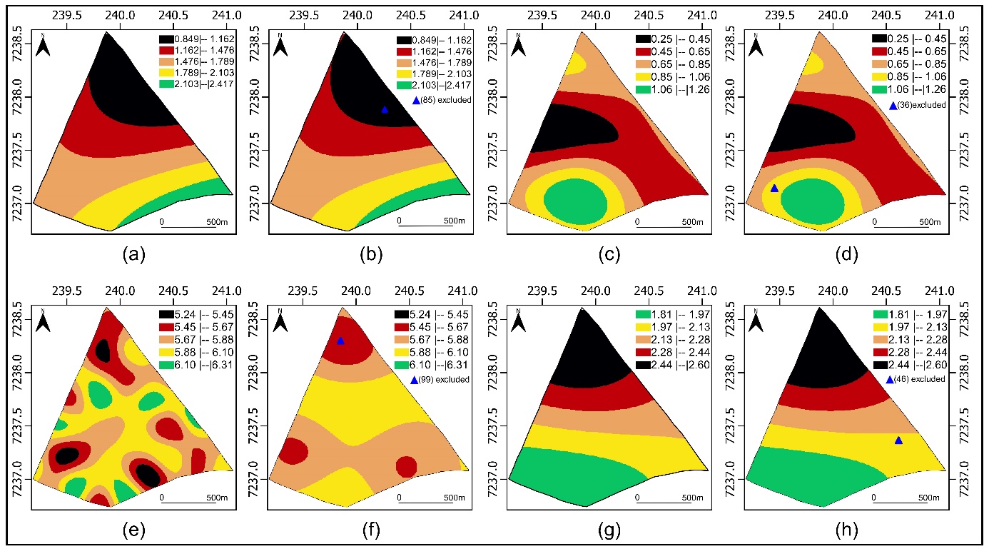
Fig 4. Thematic map of: (a) soybean productivity with all observations; (b) soybean productivity without influential observation #85; (c) copper with all observations; (d) copper without influential observation #36; (e) pH with all observations; (f) pH without influential observation #99; (g) soil penetration resistance in the layer 0.21 to 0.30 meters deep with all observations; (h) soil penetration resistance in the layer 0.21 to 0.30 meters deep without influential observation #46.
 |
 |
 |
 |
|---|---|---|---|
| (a) | (b) | (c) | (d) |
 |
 |
 |
 |
| (e) | (f) | (g) | (h) |
Fig 5. Plots of \(C_{i}\) e \(|L_{\max}|\) as a function of the order of collected observations: (a) \(C_{i}\) for soybean productivity; (b) \(|L_{\max}|\) for soybean productivity; (c) \(C_{i}\) for copper, (d) \(|L_{\max}|\) for copper; (e) \(C_{i}\) for pH, (f) \(|L_{\max}|\) for pH; (g) \(C_{i}\) for soil penetration resistance in the layer 0.21 to 0.30 meters deep; (h) \(|L_{\max}|\) or soil penetration resistance in the layer 0.21 to 0.30 meters deep.
visually observed differences in the maps. For the variables soybean productivity, soil resistance to penetration and copper content soil, a high similarity is observed between the maps considering all observations and those excluding influential observations (\({\widehat{K}}_{w} \geq 0.75\)) (Table 4). Regarding pH a modered similarity is observed between the map considering all observations and those excluding influential observation (\(0.4 < {\widehat{K}}_{w} \leq 0.75\)) (Table 4).
Materials and methods
Area study and data
The soybean productivity data (Prod) [\(t\ ha^{- 1}\)], soil Copper content (Cu) [\(mg\ dm^{- 3}\)], soil pH, and soil resistance to penetra-
tion in the layer 0.21 to 0.30 m (\(RSP_{0.21 - 0.30m}\)) [MPa] were selected due to their symmetry and normal distribution. These data were collected during the agricultural year 2022/2023 in a commercial area of 167.35 ha located in the western region of Paraná, Brazil, near the city of Cascavel, with the following geographic coordinates: latitude 24º57'18"S, longitude 53º34'29"W, and average altitude of 714 m (Figure 1). The regional climate is mesothermal and super humid temperate, climatic type Cfa (Köppen), and its soil is classified as typical Dystrophic Red Latosol with a clayey texture (Santos et al., 2018).
The 102 sampling points were defined using a lattice plus close pairs sampling approach (Diggle; Ribeiro Junior, 2007; Chipeta et al., 2017). These points were manually collected and recorded with a GPS device.
| Table 3. Spatial Dependence Index - SDI classification. | ||||
|---|---|---|---|---|
| Model | MF | Weak | Moderate | Strong |
| Wave | 0.58900 | SDI ≤ 11% | 11% < SDI ≤ 24% | SDI > 24% |
| \(SDI = MF\left( \frac{\varphi_{2}}{\varphi_{1} + \varphi_{2}} \right)\min\left\{ 1;\left( \frac{a}{0.5MD} \right) \right\} 100\), MF: Specific factor for each model, \(\varphi_{1}\): nugget, \(\varphi_{2}\): sill, a: range, MD: is the maximum distance between two sampling points. Source: (Seidel and Oliveira, 2016; Neto et al., 2018) | ||||
| Table 4. Kappa index (\(\widehat{K}\)) and weighted Kappa index (\({\widehat{K}}_{w}\)) for the comparison between the maps obtained with all observations and the maps obtained excluding the influential observations. | ||
|---|---|---|
| Comparison | \[\widehat{K}\] | \[{\widehat{K}}_{w}\] |
| Prod \(\times\) Prod#85 | 0.967 | 0.991 |
| Cu \(\times\) Cu#36 | 0.992 | 0.998 |
| pH \(\times\) pH#99 | 0.245 | 0.452 |
| \(RSP_{0.21 - 0.30m}\) \(\times\) \(RSP_{0.21 - 0.30m}\)#46 | 0.980 | 0.996 |
| Classification: \({\widehat{K}}_{w}\)≥0.75 indicates a high similarity; 0.4<\({\widehat{K}}_{w}\)<0.75 indicates moderate similarity; \({\widehat{K}}_{w}\)≤0.4 indicates low or insufficient similarity; Prod: soybean productivity with all observations; Prod#85: soybean productivity without the influential observation #85; Cu: copper with all observations; Cu#36: copper without the influential observation #36; pH#99: pH without the influential observation #99; \(RSP_{0.21 - 0.30m}\): soil penetration resistance in the 0.21 to 0.30 meters depth layer with all observations; \(RSP_{0.21 - 0.30m}\)#46: soil penetration resistance in the 0.21 to 0.30 meters depth layer without the influential observation #46. | ||
Geostatistical analysis
To model the spatial dependence structure of a regionalized variable, a stochastic process \(\mathbf{Z} = \{\mathbf{Z}(\mathbf{s}),\ \mathbf{s} \in \mathbf{S}\}\) was considered, where \(\mathbf{s} = (x,y)^{\top}\) is a vector representing a specific location in the study area \(\mathbf{S} \subset \ \mathbb{R}^{2}\), where \(\mathbb{R}^{2}\) is the two-dimensional Euclidean space. It is assumed that the data \(\mathbf{Z} = \left( Z\left( \mathbf{s}_{1} \right),\ \ldots,\ Z\left( \mathbf{s}_{n} \right) \right)^{\top}\) constitute a second-order stationary and isotropic stochastic process, collected at known locations \((\mathbf{s}_{1},\ldots,\ \mathbf{s}_{n})\), and modeled by the set \(\mathbf{Z} = \ \mu\mathbf{1} + \mathbf{\varepsilon}\), where \(\mu\) represents the constant process mean, \(\mathbf{1}\) represents a vector of ones of size \(n\ \times 1\) e \(\mathbf{\varepsilon} = \left( \varepsilon\left( \mathbf{s}_{1} \right),\ \ldots,\ \varepsilon\left( \mathbf{s}_{n} \right) \right)^{\top}\) represents the vector of random errors, \(n\ \times 1\), with a multivariate normal distribution, where \(E\left( \mathbf{\varepsilon} \right) = \mathbf{0}\) and covariance matrix \(\mathbf{\Sigma}\), \(n \times n\), where \(\mathbf{\Sigma} = \mathbf{\Sigma}\left\lbrack \left( \sigma_{ij} \right) \right\rbrack = C\left( Z\left( \mathbf{s}_{i} \right),\ Z\left( \mathbf{s}_{j} \right) \right),\ i,j = 1,\ \ldots,\ n\).
In parametric form, the covariance matrix \(\mathbf{\Sigma}\) can be defined as \(\mathbf{\Sigma} = \ \varphi_{1}\mathbf{I}_{n} + \varphi_{2}\mathbf{R}(\varphi_{3})\), where \(\mathbf{I}_{n}\) is the identity matrix , \(\varphi_{1} \geq 0\) is the parameter called nugget effect, \(\varphi_{2} \geq 0\) is the contribution parameter, \(\varphi_{3} \geq 0\) is the parameter defining the range \((a = g(\varphi_{3}))\) of the model, and \(\mathbf{R}\left( \varphi_{3} \right) = \lbrack(r_{ij})\rbrack\) is a symmetric and positive definite matrix. The elements \(r_{ij},\ \ i,j = 1,\ \ldots,\ n\) represent the association between points \(\mathbf{s}_{i}\) and \(\mathbf{s}_{j}\), where \(r_{ij} = 1\) if \(i = j\) and \(h_{ij} = 0\); \(r_{ij} = 0\) if \(i \neq j\) and \(\varphi_{2} = 0\); and \(r_{ij} = \ \varphi_{2}^{- 1}C(h_{ij})\) if \(i \neq j\) and \(\varphi_{2}^{- 1} \neq 0\), where \(C\left( h_{ij} \right) = C(Z\left( \mathbf{s}_{i} \right),\ Z(\mathbf{s}_{j}))\) is the theoretical covariance function and \(h_{ij} = \left\| \mathbf{s}_{i} - \mathbf{s}_{j} \right\|\) is the Euclidean distance between \(\mathbf{s}_{i}\) and \(\mathbf{s}_{j}\) (Uribe-Opazo et al., 2012; De Bastiani et al., 2015).
\[\widehat{\gamma}(h) = \frac{1}{2N(h)}\sum_{i = 1}^{N(h)}\left( Z\left( s_{i} + h \right) - Z\left( s_{i} \right) \right)^{2},\ \ (1)\]
where, \(\widehat{\gamma}(h)\) is the Matheron semivariance function estimator; \(N(h)\) is the number of pairs of sampled values at locations separated by the distance \(h\); \(Z\left( s_{i} + h \right)\) is the value of the variable Z at point \(s_{i} + h\); \(Z\left( s_{i} \right)\) is the value of the variable Z at the point \(s_{i}\).
The Wave model (Olea, 2006) (Equation (2)) was employed to model the spatial dependence structures, and the parameters were estimated by the maximum likelihood (ML) method. In addition to the Wave model, the Exponential, Gaussian, and Matérn family models were also employed in the analysis (Uribe-Opazo et al., 2023).
\[\gamma(h) = \left\{ \begin{matrix} \varphi_{1} + \varphi_{2}\left( 1 - \frac{\varphi_{3}}{h}sen\left( \frac{h}{\varphi_{3}} \right) \right),\ \ \ h > 0 \\ \ \ \ \ \ \ \ \ \ \ \ \ \ \ \ \ \ \ \ \ \ \ \ \ \ \ \ \ \ \ 0,\ \ \ \ \ \ \ \ \ \ \ \ \ \ \ \ \ \ \ \ \ \ \ \ h = 0 \\ \end{matrix} \right.\ \ \ ,\ \ \ \ \ \ \ \ \ \ \ (2)\]
For the Wave model, the first and second-order derivatives of the covariance structure are required \(\mathbf{\Sigma} = \ \varphi_{1}\mathbf{I}_{n} + \varphi_{2}\left( \frac{\varphi_{3}}{h}\sin\left( \frac{h}{\varphi_{3}} \right) \right)\), where: \(\frac{\partial\mathbf{\Sigma}}{\partial\varphi_{1}} = \mathbf{I}_{n}\); \(\frac{\partial\mathbf{\Sigma}}{\partial\varphi_{2}} = \mathbf{R}(\varphi_{3})\); \(\frac{\partial\mathbf{\Sigma}}{\partial\varphi_{3}} = \varphi_{2}\left\lbrack \frac{1}{h}\sin{\left( \frac{h}{\varphi_{3}} \right) - \frac{1}{\varphi_{3}}\cos\left( \frac{h}{\varphi_{3}} \right)} \right\rbrack\); \(\frac{\partial^{2}\mathbf{\Sigma}}{\partial\varphi_{1}^{2}} = 0\); \(\frac{\partial^{2}\mathbf{\Sigma}}{\partial\varphi_{1}\partial\varphi_{2}} = 0\); \(\frac{\partial^{2}\mathbf{\Sigma}}{\partial\varphi_{1}\partial\varphi_{3}} = 0\); \(\frac{\partial^{2}\mathbf{\Sigma}}{\partial\varphi_{2}^{2}} = 0\); \(\frac{\partial^{2}\mathbf{\Sigma}}{\partial\varphi_{2}\partial\varphi_{3}} = \frac{1}{h}\sin{\left( \frac{h}{\varphi_{3}} \right) - \frac{1}{\varphi_{3}}\cos\left( \frac{h}{\varphi_{3}} \right)}\); \(\frac{\partial^{2}\mathbf{\Sigma}}{\partial\varphi_{3}^{2}} = - \frac{\varphi_{2}h}{\varphi_{3}^{3}}\sin\left( \frac{h}{\varphi_{3}} \right)\).
Maximum Likelihood (ML)
A model \(Z\sim N_{n}(\mu\mathbf{1},\mathbf{\Sigma})\) with mean μ1 and covariance matrix \(\mathbf{\Sigma} = \varphi_{1}\mathbf{I}_{n} + \varphi_{2}\mathbf{R}\), which depends only on the parameter vector \(\mathbf{\varphi}\) (Diggle and Ribeiro, 2007) is considered. The logarithm of the likelihood function is defined in Equation (3) in which the vector of unknown model parameters \(\mathbf{\theta} = \left( \mu,\ \mathbf{\varphi}^{T} \right)^{T}\) and \(\mathbf{\varphi} = \left( \varphi_{1},\varphi_{2},\varphi_{3} \right)^{T}\) can be estimated by maximizing the logarithm of the likelihood function (Mardia and Marshal, 1984):
\[\mathcal{L}\left( \mathbf{\theta} \right) = - \left( \frac{n}{2} \right)\log(2\pi) - \frac{1}{2}\log\left| \mathbf{\Sigma} \right| - \frac{1}{2}\left( \mathbf{Z} - \mu\mathbf{1} \right)^{T}\mathbf{\Sigma}^{- 1}\left( \mathbf{Z} - \mu\mathbf{1} \right),\ \ \ \ \ \ \ \ (3)\]
The score functions of \(\mathbf{\theta} = \left( \mu,\ \mathbf{\varphi}^{T} \right)^{T}\) are \(U\left( \mathbf{\theta} \right) = \left( U(\mu),U(\mathbf{\varphi}) \right)\), where: \(U(\mu) = \frac{\partial\mathcal{L(}\mathbf{\theta})}{\partial\mathbf{\mu}} = \mathbf{1}^{T}\mathbf{\Sigma}^{- 1}(\mathbf{Z} - \mu\mathbf{1})\) and \(U\left( \mathbf{\varphi} \right) = \frac{\partial\mathcal{L(}\mathbf{\theta})}{\partial\mathbf{\varphi}}\) that have as their \(j\)-th elements \(\frac{\partial\mathcal{L(}\mathbf{\theta})}{\partial\varphi_{j}} = - \frac{1}{2}tr\left\{ \mathbf{\Sigma}^{- 1}\frac{\partial\mathbf{\Sigma}}{\partial\varphi_{j}} \right\} + \frac{1}{2}\mathbf{\varepsilon}^{T}\mathbf{\Sigma}^{- 1}\frac{\partial\mathbf{\Sigma}}{\partial\varphi_{j}}\mathbf{\Sigma}^{- 1}\mathbf{\varepsilon}\), \(j\)=1,2,3 and \(\mathbf{\varepsilon} = \left( \mathbf{Z} - \mu\mathbf{1} \right)\).
To estimate the parameters μ and φ, we solve the systems of equations\(\ U(\mu) = 0\) and \(U\left( \mathbf{\varphi} \right) = \mathbf{0}\). The observed information matrix is defined by \(\mathcal{L}\left( \mathbf{\theta} \right) = - \mathbf{L}(\mathbf{\theta})\) and should be evaluated at \(\mathbf{\theta} = \widehat{\mathbf{\theta}}\), its partitioned form is \(\mathbf{L}\left( \mathbf{\theta} \right) = \begin{pmatrix} \mathbf{L}_{\mu\mu} & \mathbf{L}_{\mu\mathbf{\varphi}} \\ \mathbf{L}_{\mathbf{\varphi}\mu} & \mathbf{L}_{\mathbf{\varphi\varphi}} \\ \end{pmatrix}\) where, \(\mathbf{L}_{\mu\mu} = \frac{\partial^{2}\mathcal{L}\left( \mathbf{\theta} \right)}{\partial\mu\partial\mu^{T}} = - \mathbf{1}^{T}\mathbf{\Sigma}^{- 1}1\); \(\mathbf{L}_{\mu\mathbf{\varphi}} = \mathbf{L}_{\mathbf{\varphi}\mu}^{T} = \frac{\partial^{2}\mathcal{L}\left( \mathbf{\theta} \right)}{\partial\mu\partial\mathbf{\varphi}^{T}}\), with elements \(\frac{\partial^{2}\mathcal{L}\left( \mathbf{\theta} \right)}{\partial\mu\partial\varphi_{j}} = - \mathbf{1}^{T}\mathbf{\Sigma}^{- 1}\frac{\partial\mathbf{\Sigma}}{\partial\varphi_{j}}\mathbf{\Sigma}^{- 1}\mathbf{\varepsilon}\), \(j = 1,\ldots,q\); where, \(\mathbf{\varepsilon} = (\mathbf{Z} - \mu\mathbf{1})\), and \(\mathbf{L}_{\mathbf{\varphi\varphi}} = \frac{\partial^{2}\mathcal{L}\left( \mathbf{\theta} \right)}{\partial\mathbf{\varphi}\partial\mathbf{\varphi}^{T}}\), with elements \(\frac{\partial^{2}\mathcal{L}\left( \mathbf{\theta} \right)}{\partial\varphi_{i}\partial\varphi_{j}} = \frac{1}{2}tr\left\{ \mathbf{\Sigma}^{- 1}\left( \frac{\partial\mathbf{\Sigma}}{\partial\varphi_{i}}\mathbf{\Sigma}^{- 1}\frac{\partial\mathbf{\Sigma}}{\partial\varphi_{j}} - \frac{\partial^{2}\mathbf{\Sigma}}{\partial\varphi_{i}\partial\varphi_{j}} \right) \right\} + \frac{1}{2}\mathbf{\varepsilon}^{T}\mathbf{\Sigma}^{- 1}\left\{ \frac{\partial^{2}\mathbf{\Sigma}}{\partial\varphi_{i}\partial\varphi_{j}} - \frac{\partial\mathbf{\Sigma}}{\partial\varphi_{i}}\mathbf{\Sigma}^{- 1}\frac{\partial\mathbf{\Sigma}}{\partial\varphi_{j}} - \frac{\partial\mathbf{\Sigma}}{\partial\varphi_{j}}\mathbf{\Sigma}^{- 1}\frac{\partial\mathbf{\Sigma}}{\partial\varphi_{i}} \right\}\mathbf{\Sigma}^{- 1}\mathbf{\varepsilon}\), \(i,j = 1,\ldots,q\). In this work \(q = 3\).
The expected information matrix is of the form \(\mathbf{K}\left( \mathbf{\theta} \right) = E\lbrack - \mathbf{L}(\mathbf{\theta})\rbrack\), It is a diagonal matrix of the form \(\mathbf{K}\left( \mathbf{\theta} \right) = \begin{pmatrix} \mathbf{K}(\mu) & \mathbf{0} \\ \mathbf{0} & \mathbf{K}(\mathbf{\varphi}) \\ \end{pmatrix}\), where \(\mathbf{K}(\mu) = E\left\lbrack - \mathbf{L}_{\mu\mu} \right\rbrack = E\left\lbrack - \frac{\partial^{2}\mathcal{L}\left( \mathbf{\theta} \right)}{\partial\mu\partial\mu^{T}} \right\rbrack = \mathbf{1}^{T}\mathbf{\Sigma}^{- 1}\mathbf{1}_{n}\) and \(\mathbf{K}\left( \mathbf{\varphi} \right) = E\left\lbrack - \mathbf{L}_{\mathbf{\varphi\varphi}} \right\rbrack = E\left\lbrack - \frac{\partial^{2}\mathcal{L}\left( \mathbf{\theta} \right)}{\partial\mathbf{\varphi}\partial\mathbf{\varphi}^{T}} \right\rbrack\), Its elements are \(k_{ij}(\varphi) = \frac{1}{2}tr\left\lbrack \mathbf{\Sigma}^{- 1}\frac{\partial\mathbf{\Sigma}}{\partial\varphi_{i}}\mathbf{\Sigma}^{- 1}\frac{\partial\mathbf{\Sigma}}{\partial\varphi_{j}} \right\rbrack\), with \(i,j = 1,\ldots,q\) (Uribe-Opazo et al., 2012).
The asymptotic standard errors can be calculated by inverting the information matrix \(\mathbf{K}\left( \mathbf{\theta} \right)^{- 1}\) and taking the square root of the diagonal elements (Uribe-Opazo et al., 2012; 2023).
Local influence
De Bastiani et al. (2015) proposed a generalized perturbation on the response variable \(\mathbf{Z}_{\omega} = \mathbf{Z} + \mathbf{\Sigma}^{\frac{1}{2}}\omega\) where \(\omega\) is a vector belonging to the perturbation space \(\Omega\). The logarithm of the perturbed likelihood function for the normal model is given by:
\(\mathcal{L}\left( \mathbf{\theta}_{\omega} \right) = \mathcal{L}\left( \mathbf{\theta}|\mathbf{\omega} \right) = - \left( \frac{n}{2} \right)\log(2\pi) - \frac{1}{2}\log\left| \mathbf{\Sigma} \right| - \frac{1}{2}\left( \mathbf{Z}_{\mathbf{\omega}} - \mu\mathbf{1} \right)^{T}\mathbf{\Sigma}^{- 1}\left( \mathbf{Z}_{\mathbf{\omega}} - \mu\mathbf{1} \right)\).
In this study, the matrix \(\mathbf{\Delta} = \left( \mathbf{\Delta}_{\mu}^{T},\ \mathbf{\Delta}_{\varphi}^{T} \right)^{T}\) evaluated in \(\mathbf{\theta} = \widehat{\mathbf{\theta}}\) and in \(\mathbf{\omega} = \mathbf{\omega}_{0}\), is of the form \(\mathbf{\Delta}_{\mu} = - \mathbf{1}_{n}^{T}\mathbf{\Sigma}^{- 1}\mathbf{\Sigma}^{\frac{1}{2}}\); \(\mathbf{\Delta}_{\varphi} = \frac{\partial^{2}\mathcal{L}\left( \mathbf{\theta}|\mathbf{\omega} \right)}{\partial\mathbf{\varphi}\partial\mathbf{\omega}^{T}}\), that has as elements \(\mathbf{\mathrm{\Delta}}_{\varphi_{\mathbf{j}}} = \mathbf{\varepsilon}^{T}\left\lbrack \mathbf{\Sigma}^{- 1}\frac{\partial\mathbf{A}}{\partial\varphi_{j}} - \mathbf{D}_{j}\mathbf{A} \right\rbrack\), to \(j = 1,\ldots,q\), where \(\mathbf{A} = \mathbf{\Sigma}^{\frac{1}{2}}\), \(\mathbf{\varepsilon} = \mathbf{\varepsilon}\left( \mathbf{\omega}_{0} \right) = (\mathbf{Z} - \mu\mathbf{1})\), and \(\mathbf{D}_{j} = \mathbf{\Sigma}^{- 1}\frac{\partial\mathbf{\Sigma}}{\partial\mathbf{\varphi}_{j}}\mathbf{\Sigma}^{- 1}\).
Consider the matrix \(\mathbf{B} = \mathbf{\Delta}^{T}\mathbf{L}^{- 1}\mathbf{\Delta}\) where, \(\mathbf{L}\) is the observed information matrix, and the element \(C_{i} = 2\left| b_{ii} \right|\), for \(i = 1,\ldots,n\), where \(b_{ii}\) is the element of the main diagonal of matrix \(\mathbf{B}\). From matrix \(C_{i}\) as a function of 𝑖 (order of observations) can be used as a diagnostic technique to assess the existence of influential observations.
Let \(L_{\max}\) be the normalized eigenvector associated with the largest eigenvalue in absolute value of matrix 𝐵. According to Cook (1986) the chart of the elements \(\left| L_{\max} \right|\) as a function of 𝑖 (order of observations) can reveal the elements that, under small perturbations, exert the greatest influence on the likelihood deviation.
Comparisons
The measure of the degree of spatial dependence of the fitted models was obtained through the Spatial Dependency Index (SDI) (Seidel and Oliveira, 2014), classified according to Table 3 (Seidel and Oliveira, 2016; Neto et al., 2018). This classification is essential for interpreting the results and making decisions based on the spatial dependence analysis in the fitted models.
The similarity between the interpolated maps was assessed by estimating the Kappa (\(\widehat{K}\)) and weighted Kappa \(\left( {\widehat{K}}_{w} \right)\) (Cohen, 1960;1968). The weighted Kappa index \(\left( {\widehat{K}}_{w} \right)\) is relies on weights \(w_{ij}\) to quantify differences. The classification of the weighted Kappa index is equivalent to the Kappa index (Table 4) (Fleiss et al., 2003).
Computational resources
All the analyses were performed using the R software (R Core Team, 2023). Semivariances were calculated using functions from the geoR package, which was also employed to fit the models and produce thematic maps (Ribeiro Junior and Diggle, 2001). The vcd package was used to calculate the weighted Kappa index (Meyer et al., 2021).
Conclusion
The Wave model stood out compared to other models, being the most appropriate for characterizing the spatial dependence structure of soybean productivity and soil attributes for the year under study. The generated maps not only enabled the prediction of variables in unsampled locations within the study area but also allowed for the creation of differentiated management zones, considering productivity and soil properties. This approach enables the localized application of inputs, aiming to maximize economic return and minimize environmental impacts, resulting in efficient agro-management.
Furthermore, the identification and removal of influential observations caused changes in the parameter estimates that define the spatial dependence structure, directly impacting the characteristics of the sectors of the maps of soybean productivity and soil attributes. The importance of conducting local influence diagnostic studies in geostatistical analyses is emphasized to ensure the robustness and accuracy of the obtained results.
Worthy of note is the potential applicability of the methodology presented in this work for studying the productivity of other crops and different soil attributes in various areas and over different periods, thus expanding its scope and relevance in the context of precision agriculture and sustainable and rational management of natural resources.
Acknowledgment
Council for Scientific and Technological Development (CNPq); Coordination for the Improvement of Higher Education Personnel (CAPES) , Financing Code 001; Post-Graduate Program in Agricultural Engineering of Western State University of Paraná (PGEAGRI-UNIOESTE); Federal Technological University of Paraná (UTFPR) and Spatial Statistics Laboratory (LEE-UNIOESTE).
References
Akaike H (1973) Information theory and an extension of the maximum likelihood principle. Stat-J Roy St. 51:469-483.
Amirinejad AA, Kamble K, Aggarwal P, Chakraborty D, Pradhan S, Mittal RB (2011) Assessment and mapping of spatial variation of soil physical health in a farm. Geoderma. 160:292-303.
Canarache A (1990) A generelized semi-empirical model estimating soil resistence to penetration. Soil Till Res. 16(01):51-70
Carvalho JRP de, Vieira SR, Greco CR (2009) Comparação de métodos para ajuste de modelos de semivariograma da precipitação pluvial anual. Rev Bras Eng Agr Amb. 13(4):443-448.
Chipeta MG, Terlouw DJ, Phiri KS, Diggle PJ (2017) Inhibitory geostatistical designs for spatial prediction taking account of uncertain covariance structure. Environmetrics. 28(1):2425.
Clark I (1979) Practical geostatistics. London: Applied Science Publishers. 20 p.
Cohen J (1960) A coefficient of agreement for nominal scales. Educ Psychol Meas. 20(1):37-46.
Cohen J (1968) Weighted kappa: nominal scale agrément with provision for scale disagreement or partial credit. Psychol Bull. 70(4):213-220.
Conab (2021) Séries históricas: soja Brasil – série histórica de produtividade – safras 1976/1977 a 2022/2023. < https://www.conab.gov.br/info-agro/safras/serie-historica-das-safras?start=30 >.
Cook RD (1986) Assessment of local influence. Stat-J Roy St. 48(2):133–169.
Cressie N (2015) Statistics for spatial data. New York: John Wiley & Sons. 928 p.
Dalposso GH, Uribe-Opazo MA, De Bastiani F (2021) Spatial-temporal Analysis of Soybean Productivity Using Geostatistical Methods. Journal of Agricultural Studies. 9(2):283-303.
Dalposso GH, Uribe-Opazo MA, Oliveira MP de (2022) Comparison between Matheron and Genton semivariance function estimators in spatial modeling of soybean yield. Aust J Crop Sci. 16(07):916-921.
De Bastiani F, Cysneiros AHMD, Uribe-Opazo MA, Galea M (2015) Influence diagnostics in elliptical spatial linear models. Test. 24(2):322–340.
Diggle PJ, Ribeiro Junior PJ (2007) Model based Geoestatístics. New York: Springer.
Fagundes RS, Uribe-Opazo MA, Guedes LPC, Galea M (2018) Slash spatial linear modeling: soybean yield variability as a function of soil chemical properties. Rev Bras Cienc Solo. 42:0170030.
Faraco MA, Uribe-Opazo MA, Silva EAA, Johann JA, Borssoi JA (2008) Seleção de modelos de variabilidade espacial para a elaboração de mapas temáticos de atributos físicos do solo e produtividade da soja. Rev Bras Cien Solo. 32(02):463-476.
Fleiss JL, Levin B, Myunghee C P (2003) Statistical methods for rates and proportions. 3rd edn. New Jersey: John Wiley. 800 p.
Guedes LPC, Uribe-Opazo MA, Ribeiro Junior PJ (2013) Influence of incorporating geometric anisotropy on the construction of thematic maps of simulated data and chemical attributes of soil. Chil J Agr Res. 73(4):414–423.
Hansch R, Mendel RR (2009) Physiological functions of mineral micronutrientes (Cu, Zn, Mn, Fe, Ni, Mo, B, Cl). Curr Opin Plant Biol. 12:259-266.
Isaaks EH, Srivastava RM (1989) An introduction to applied geostatistics. New York: Oxford University Press, 560 p.
Keller T, Sandin M, Colombi T, Horn R, Or D (2019) Historical increase in agricultural Machinery weights enhanced soil stress levels and adversely affected soil functioning. Soil Till Res. 194:104293.
Leiva V, Sánchez L, Galea M, Saulo H (2020) Global and local diagnostic analytics for a geostatistical model based on a new approach to quantile regression. Stoch Env Res Risk A. 34:1457–1471.
Lorbieski R, Guedes LPC, Uribe-Opazo MA, Kestring FBF (2023) Regionalization of an agricultural area by means of multivariate data and their relationship with soybean productivity. Aust J Crop Sci. 17(7):570-580.
Mahdi E, Abuzaid AH, Atta, AMA (2020) Empirical variogram for achieving the best valid variogram. Commun Stat Appl Methods. 27:547-568.
Maltauro TC, Guedes LPC, Canton LED, Uribe-Opazo MA (2023) Spatial multivariate optimization for a sampling redesign with a reduced sample size of soil chemical properties. Rev Bras Cien Solo. 47:0220072.
Mardia KV, Marshal RJ (1984) Maximum likelihood estimation of models for residual covariance in spatial regression. Biometrika. 71(01):135-146.
Meyer D, Zeileis A, Hornik K (2021) Package “vcd”: visualizing categorical data. R Package Version. 1:4-9. <https://CRAN.R-project.org/package=vcd>.
Neto EA, Barbosa IC, Seidel EJ, Oliveira MS de (2018) Spatial dependence index for cubic, pentaspherical and wave semivariogram models. Bulletin of Geodetic Sciences. 24(01):142-151.
Olea RA (2006) A six-step practical approach to semivariogram modeling. Stoch Env Res Risk A. 20(5):307-318.
Oliver MA (2010) Geostatistical Applications for Precision Agriculture. Dordrecht: Springer. 331 p.
Ribeiro Junior PJ, Diggle PJ (2001) geoR: A package for geostatistical analysis. R News. 1(2):15–18.
R Core Team (2023) R: A language and environment for statistical computing. R Foundation for Statistical Computing, Vienna, Austria. <https://www.R-project.org>.
Santos DR, Silva, LS (2001) Fertilidade do solo e nutrição de plantas. Santa Maria: Universidade Federal de Santa Catarina, 20 p.
Santos HG, Jacomini PKT, Anjos LHC, Oliveira VA, Lumbreras JF, Coelho MR, Almeida JA, Araújo Filho JC, Oliveira JB, Cunha TJF (2018) Sistema Brasileiro de classificação de solos. Brasília, DF: Embrapa.
Santra P, Chopra UK, Chakraborty D (2008) Spatial variability of soil properties and its application in predicting surface map of hydraulic parameters in an agricultural farm. Curr Sci. 95(7):937-945.
Seidel EJ, Oliveira MS (2014) Novo índice geoestatístico para a mensuração da dependência espacial. Rev Bras Cienc Solo. 38:699-705.
Schwarz G (1978) Estimating the dimensiono f a model. The Annals of Statistics. 6(02):461-464.
Uribe-Opazo MA, Borssoi J, Galea M (2012) Influence diagnostics in Gaussian spatial linear models. J Appl Stat. 39(3):615–630.
Uribe-Opazo MA, De Bastiani F, Galea M, Schemmer R, Assumpção RAB (2021) Influence diagnostics on a reparametrized t-Student spatial linear model. Spatial Statistics. 41:100481.
Uribe-Opazo MA, Dalposso GH, Galea M, Johann JA, De Bastiani F, Moyano ENC, Grzegozewski DM (2023) Spatial variability of wheat yield using the gaussian spatial linear model. Aust J Crop Sci. 17(2):179-189.
Vanderhasselt A, Cool S, D’House T, Cornelis W (2023) How tine characteristics of subsoilers affect fuel consumption, penetration resistance and potato yield of a sandy loam soil. Soil Till Res. 228:105631.
Zain M, Ma H, Rahman SU, Nuruzzaman M, Chaudhary S, Azeem I, Mehmood F, Duan A, Sun C (2024) Nanotechnology in precision agriculture: advancing towards sustainable crop production. Plant Physiol Bioch. 206:108244.